Baseball catcher

This project was part of a class project for the Robotic Vision class at BYU.

Introduction

The baseball catcher project consists of using a stereo camera system to estimate the trajectory of a baseball pitched from a ptiching machine at 55 mph from about 42 feet away. After detecting and estimating the trajectory of the baseball, commands are sent to a catcher system in order to move it to the final location of the baseball, thus catching the ball.

To accomplish this, we have about 0.5 seconds (about 30 frames) to detect the baseball and estimate its trajectory before it goes out of frame and reaches the catcher system. Our solution needed to process each stereo image pair and issue commands in less than 16ms (the frame rate).

Results

On our best run, we were able to catch 20/21 pitches, with one rim shot. A rim shot is where the baseball hit the rim of the catcher system either due to the catcher still moving or an incorrect final estimate.

An shortened video of all 21 pitches is below.

Video credit: Ben Boyack

Pitches that fell outside of the region where the catcher could move (i.e. the catchable region) were ignored. Since it was hard to pitch the baseballs through the pitcher consistently, this happened several times.

An unedited video of all 21 pitches can be found here. Note that sections where we collect the balls are sped up, but no frames are taken out.

My specific contributions

This project was a collaborative effort between myself and one other student. We decided to approach this problem by independently developing image processing methods and 3D trajectory estimation algorithms, and then selecting the methods that yielded the best results.

We ended up using the image processing algorithm and the trajectory estimation algorithms that I designed. Each of these parts is described below.

Methods

To catch the baseball, we had to process each image to detect where the baseball was in the image. Instead of searching through the whole image, we defined a region of interest (ROI) where the ball was located and searched that smaller window for the ball’s location. The ROI was defined to reduce the computation time for each frame and to reduce false ball detections caused by noise or other movement. After detecting the baseball, we needed to compute the 3D position of the baseball. The trajectory of the ball could then be computed from the 3D position.

Our algorithm divided the process into five stages, ball detection, moving the ROI, 3D position estimation, trajectory estimation, and moving the catcher. The following sections detail each step.

Ball Detection

For this stereo setup, we acquired a pair (left and right) of images at each timestep. Each image was processed to detect the baseball.

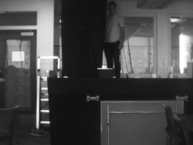
Finding the ball in an image reduces to finding a single moving circle in an almost static scene. To do this, we first took a grayscale image of the scene without the baseball present, which we used as the background image. Figure 1 shows a background image and an image captured during a launch for a test run.

Example images captured from the right camera during a launch.

Every additional grayscale frame captured was differenced from the background image using OpenCV’s absdiff method. After differencing, the image was thresholded using a binary threshold. A low threshold of 25 was chosen, meaning that every pixel in the grayscale image that had a value greater than 25 was set to 255, while every other pixel was set to 0. This thresholded image was then used to find the center of the baseball. Figure 2 shows an example of each stage of the preprocessing we performed on the ROI of each image.

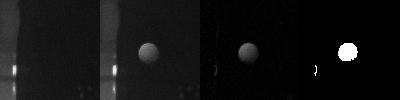
Figure 2: Method for preprocessing the image before extracting the location of the center of the ball. The background image (left) is subtracted from the current image (middle-left) to produce the absolute difference image (middle-right), which is then thresholded to produce the final preprocessed output (right).

The thresholded image was first blurred with a Gaussian blur kernel using OpenCV’s GaussianBlur function. This was done to reduce noise and jagged, disjoint contours. The Canny edges were then found, and they were passed into OpenCV’s findContours function to find the contours. We found the best results by using the RETR_FLOODFILL method in the findContours method, so that the method returned closed, external contours.

The contours found were disjoint, however, so the contours returned were then selectively merged to find the overall contour of the baseball. The process for merging contours is as follows:

Merge the contour into the previous contour to form a candidate contour.
Get the minimum enclosing circle of the circle, defined by a center and radius, with minEnclosingCircle.
If the area of the minimum enclosing circle increased larger than a threshold, or if the location of the center of the circle moved larger than another threshold, then reject the candidate contour (don’t merge it into the final contour).
Continue until all contours are merged and return the center and radius of the baseball.

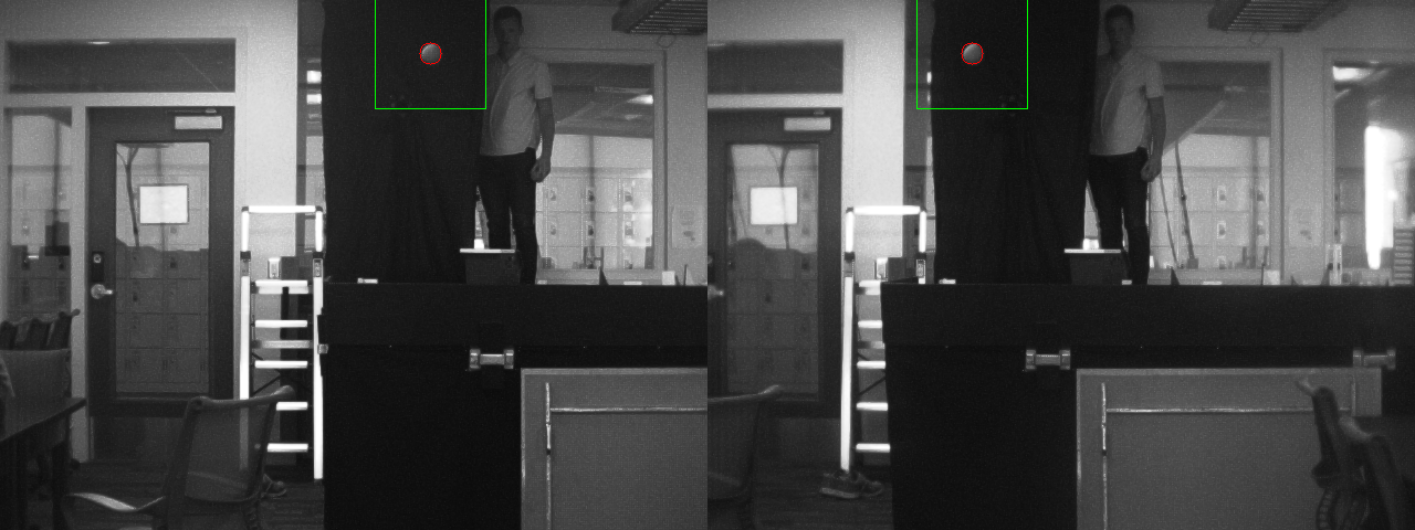
Merging the contours in this manner produced a fairly robust detection of the center and radius of the baseball. Figure 3 shows an example image with each stage of the contour detection and merging process. Note the extraneous contours in the bottom left of the image which were filtered out by the contour-merging algorithm, highlighting the robustness of our method. Figure 4 shows a stereo pair with the ROI and baseball detection labeled.

Figure 3: Method for robustly finding the center and radius of the baseball. A Gaussian blur was first performed to smooth the images (left), which was then used to find Canny edges (middle-left), which was then used to detect contours (middle-right). These contours were then merged into a single contour (represented by a set of points in the right image).

Figure 4: Stereo pair with the ROI (green) and baseball-detection circle (blue) labeled. The blue circle tracking the baseball shows that our baseball detection method worked.

Moving the ROI

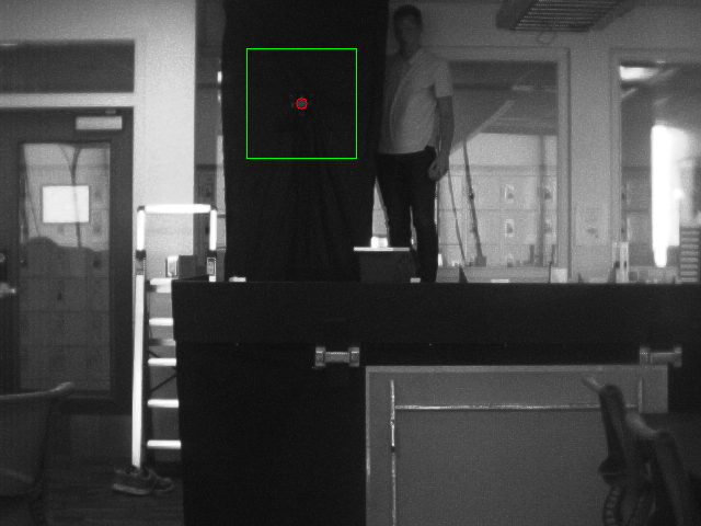
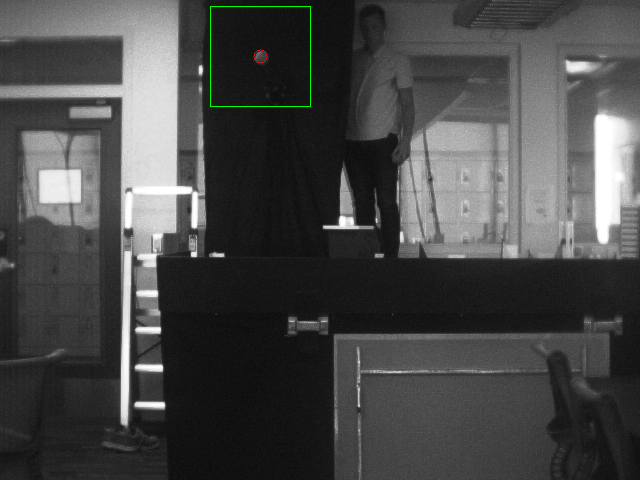
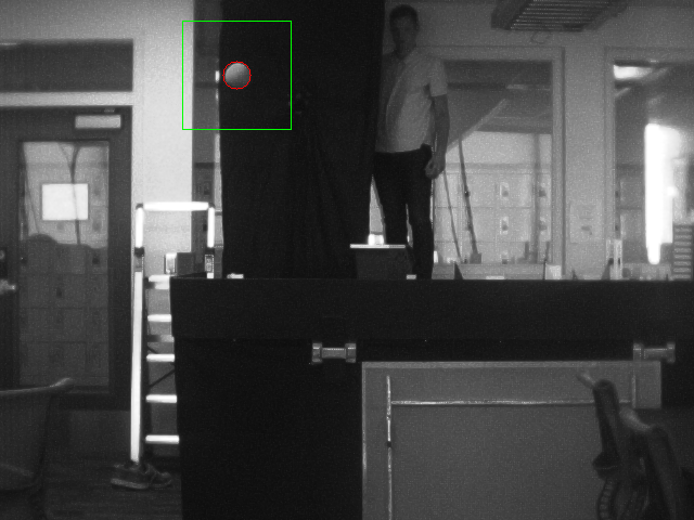
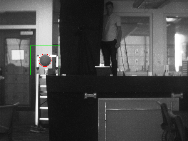
The ROI was chosen to reduce search time when detecting the baseball and to reject false ball detections. Since the ROI is a smaller subset of the image, the ball can move out of the ROI if it is not updated. To avoid this, after finding the baseball in each image, we moved the ROI so the previously detected baseball was at the center of the new ROI. The size of the ROI was tuned so that the ball did not move out of the ROI throughout the duration of the launch. We chose the side length of the ROI to be 100 pixels, which worked well for this application. Figure 5 shows a series of images from a test launch with the updated ROI marked in green.

Figure 5: Series of images from the right camera from an example launch showing how the ROI (green) moves to keep the ball detection (red) in the center of the ROI.

3D Position Estimation

After detecting the baseball in both the left and right images, we first undistorted the detected points using OpenCV’s undistortPoints function. We then triangulated the 3D position of the baseball using OpenCV’s triangulatePoints function. Note that both of these functions required parameters from individual camera calibration and stereo calibration functions, including the camera intrinsics and distortion parameters, as well as the rectification parameters and the essential matrix (rotation and translation between left and right cameras). These calibrations were performed offline and the coefficients were loaded at runtime.

The result of these two functions was a 3D estimate (XYZ) of the ball location relative to the left camera coordinate frame, expressed in the left camera’s frame.

Trajectory Estimation

The catcher could not move instantaneously. Additionally, the stereo camera system only had view of the baseball for the first 3/4 of the ball’s trajectory. Therefore, estimating the trajectory of the baseball and its final location was essential in order to successfully catch the ball.

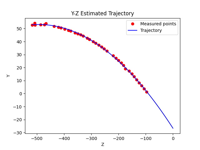
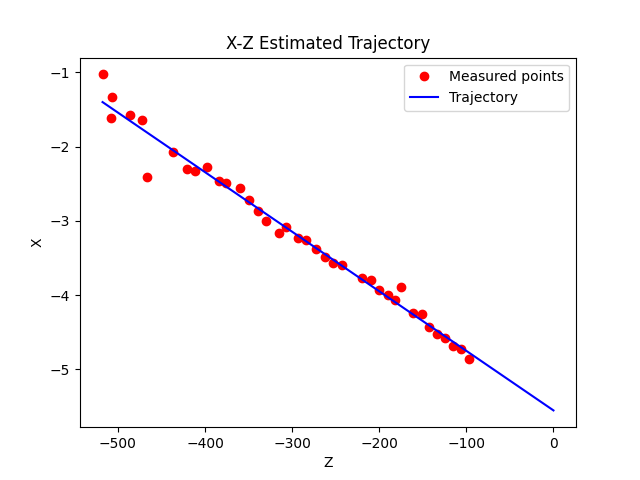
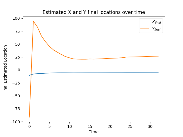
Ignoring air resistance and any spin on the baseball, the kinematics of the baseball are parabolic in the Y-Z (vertical) plane of the camera coordinate system and linear in the X-Z (horizontal) plane. After collecting at least 5 estimates of the ball’s 3D location from consecutive frames, we fit a parabola to the Y-Z data points and a straight line to the X-Z data points. We could then evaluate those fits at Z=0 to determine the final location of the baseball as it passed underneath the cameras. Figure 6 shows the estimated X-Z plane and Y-Z plane trajectories based on the measured points, as well as the estimated final location of the baseball over time as the polynomial fit improves. Note that the final estimated location stabilizes after about 10 baseball detections.

Note that to then catch the ball, we had to convert the baseball’s estimated final location from the left camera coordinate system to the stereo coordinate system and then to the catcher coordinate system. This coordinate transformation included some offset values that we tuned to remove bias or other errors in our system.

Figure 6: Measured ball locations in inches, estimated trajectories, and estimated final X-Y location of the baseball over time (in inches).

Moving the catcher

The catcher system consists of two motors with encoders. The encoders allow the system to precisely control the position of the catcher head. Our code interfaced with the catcher system by sending position commands over a serial port to the motor driver boards. An internal PID control scheme drove the catcher head to the desired location.

While powerful, the catcher system could not instantaneously move the head of the catcher to the desired location. Because of the delay between the time that we sent the desired position command and when the catcher achieved that position, it was essential that we started to move the catcher as soon as we had a good estimate. As shown in Figure 6, the estimated trajectory stabilized after about 10 measured data points. We chose to send catcher position commands after receiving 10, 20, and 30 measured baseball data points. This allowed the catcher to achieve the desired position and also did not overflow the serial buffer (which could happen by sending commands too fast).

Disclosure: I wrote this report as part of the project assignment.